Data Skies

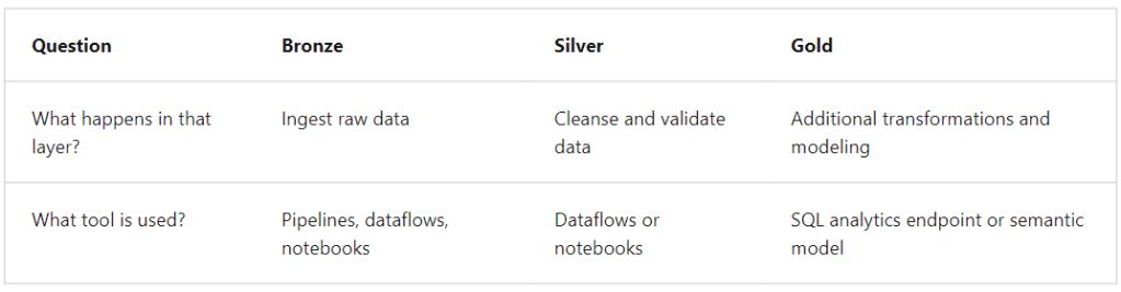
Tutorial Part 1 of 2: Implementing the Bronze Layer and Silver Layer

This article will be split over 2 parts, in this first part we get familiarized with the medallion architecture and it’s structure followed by a tutorial on how to ingest data into the first layer i.e. the bronze layer. Then, we will look into the second layer of the medallion architecture, the silver layer and learn about best practices on cleaning and validating data.

In part 2 of our tutorial, we will delve into additional transformations, modelling of data and finally setting up our data for reporting, analytics, and Data Science, including ML modelling, in the third and final layer, the Gold layer.

What is the medallion lakehouse architecture?

A medallion architecture is a data design pattern and the most popular framework that provides an approach to organizing data. First coined by Databricks, it’s now widely adapted by Microsoft to describe stages of data processing within Microsoft Fabric. The goal is to purposely increment and improve data as it flows through each layer of the architecture. As an enterprise, you would like to keep raw data as-is to fallback to at any time in your analytics journey. Your final consumers of data should only interact with the transformed and modelled data. And, in the interim, you have your data transformations and modelling. So the flow goes likes this, raw data-> transformations -> curated data.

So, how do you implement a medallion architecture? In stages! First layer, is always the bronze layer, this is where we ingest raw data. In the second layer, we cleanse and validate our data, this is called the silver layer, and finally the gold layer as this is the end point where business users interact with the data. We don’t always have to stick to these three stages, you can always add more stages to fit your own business needs.

Let’s get started with the tutorial

For this article, let’s use a CRM Sales Opportunity dataset that I found on Maven Analytics. This data includes information on accounts, products, sales teams, and sales opportunities for a fictious company that sells computer hardware. We are going to use this data set for our tutorial and learn how we can implement medallion architecture in Microsoft Fabric.

Take a look at the overall architecture for this project and review the different stages involved in the process.

Create a Lakehouse and upload data to bronze layer

Navigate to app.powerbi.com

• Create a workspace and call it ‘Medallion’ with Fabric trial instance enabled in it.
• Once complete, navigate to the workspace setting and enable the Data modelling setting. This will ensure we are able to create relationships in our semantic model.

• Create a new Lakehouse in the Medallion workspace and call it ‘Sales’.
• Download the data file for this tutorial from https://mavenanalytics.io/data-playground. Extract the files and save it to your local folders.
• Navigate to the Data Lakehouse explorer pane and create a new folder ‘Bronze’ under the Files folder.
• Select the Upload files option to ingest our downloaded files into the lakehouse.

• Once the upload is complete, you should see all the related csv files under the CSV files folder.

Our first stage of importing data into the lakehouse for the purposes of implementing a medallion architecture is now complete and we have achieved the bronze layer.

Transform data and load into Delta tables for Silver layer

Now that we have some files in our bronze layer of our lakehouse, let’s use a notebook to transform this data and load into delta tables.

• From within your workspace, select Notebook under the Data Science section and let’s name it as ‘Transform Data for Silver layer’.
• Select the existing cell in the notebook, highlight all the codes and delete the lines.
• Using the codes below, we read data from our files in the bronze layer, perform necessary transformations and save data as delta tables into the lakehouse. This marks the completion of our second stage in the medallion architecture, the silver layer. Our data is now ready to be loaded into the third and final layer, the gold layer.
• In your lakehouse, you will now see all your raw files in the Bronze layer, under folders, and the transformed data in the silver layer, under tables.

##### Define the data schema for accounts table. 
##### Remove null values in subsidiary_of by** None **values. 
##### Adding a created on field to store a time stamp of when the data was created. 

from pyspark.sql.types import *
from pyspark.sql.functions import when, lit, col, current_timestamp, input_file_name
from pyspark.sql.functions import to_timestamp

df = spark.read.format("csv").option("header", "true").load("Files/Bronze/accounts.csv")
df = df.withColumn("account", df["account"].cast("string"))
df = df.withColumn("sector", df["sector"].cast("string"))
df = df.withColumn("year_established", df["year_established"].cast("double"))
df = df.withColumn("revenue", df["revenue"].cast("float"))  # Adjust scale and precision as needed
df = df.withColumn("employees", df["employees"].cast("double"))
df = df.withColumn("office_location", df["office_location"].cast("string"))
df = df.withColumn("subsidiary_of", df["subsidiary_of"].cast("string"))  
df = df.withColumn("subsidiary_of", col("subsidiary_of").cast("string")) \
    .fillna({"subsidiary_of": "None"})
df = df.withColumn("created_on", current_timestamp())

##### Define the delta table for accounts table. 

from delta.tables import *
DeltaTable.createIfNotExists(spark) \
     .tableName("account_silver") \
     .addColumn("account", StringType()) \
     .addColumn("sector", StringType()) \
     .addColumn("year_established", DoubleType()) \
     .addColumn("revenue", FloatType()) \
     .addColumn("employees", DoubleType()) \
     .addColumn("office_location", StringType()) \
     .addColumn("subsidiary_of", StringType()) \
     .addColumn("new_created_on",TimestampType()) \
     .execute()

##### Write all records from df to the delta table. 

df.write.mode("overwrite").option("overwriteSchema", "true").saveAsTable("account_silver")

##### Define the data schema for the data_dictonary table. 

df = spark.read.format("csv").option("header","true").load("Files/Bronze/data_dictionary.csv")

df.write.mode("overwrite").saveAsTable("silver_data_dictonary")

##### Define the data schema for the products table. 

df = spark.read.format("csv").option("header","true").load("Files/Bronze/products.csv")
df = df.withColumn("sales_price", df["sales_price"].cast("double"))

df.write.mode("overwrite").saveAsTable("silver_products")

##### Define the data schema for the sales team table. 

df = spark.read.format("csv").option("header","true").load("Files/Bronze/sales_teams.csv")

df.write.mode("overwrite").saveAsTable("silver_sales_teams")

##### Define the data schema for the sales pipeline table. 

df = spark.read.format("csv").option("header","true").load("Files/Bronze/sales_pipeline.csv")
df = df.withColumn("engage_date", df["engage_date"].cast("date"))
df = df.withColumn("close_date", df["close_date"].cast("date"))
df = df.withColumn("close_value", df["close_value"].cast("float"))
df = df.withColumn("close_value", col("close_value").cast("float")) \
    .fillna({"close_value": "0"})
df = df.withColumn("account", col("account").cast("string")) \
    .fillna({"account": "None"})

df.write.mode("overwrite").saveAsTable("silver_sales_pipeline")

Additional Points

1. Microsoft recommends as best practice to create a lakehouse for each layer, in it’s own separate Fabric workspace. For this tutorial, since we are using a basic data model, we will be using only one workspace and one lakehouse for the whole process.
2. For our data ingestion model, we use the explorer pane to upload files into our Bronze layer, this ingestion could have been achieved using dataflows or pipelines too but given the simplicity of our model we used the basic upload files option.
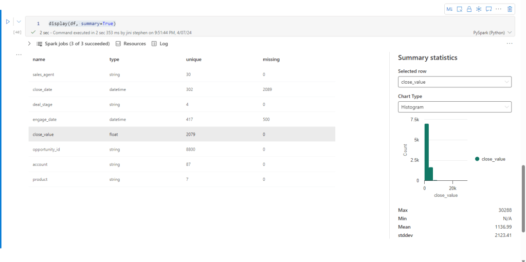
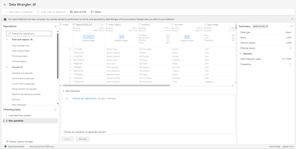
3. You wouldn’t always know what transformations to use on your tables to prepare the data for the silver layer. So, once you have loaded the data into a dataframe, you can run this code display(df, summary=True) in your notebook and get the summary statistics. There’s also the Data Wrangler that will not only help you summarize your data but also make live transformations. This will be a future article for sure.

So, this ends our Part 1 of 2 tutorials.

In our next article, we will look into the Gold layer of our medallion architecture and see how we can use it as an endpoint for the end users.

See you all in the next article 🙂